Comet_maths Interpolation Module

In this section we explain how comet_maths can be used to interpolate between different datapoints. The comet_maths interpolation module can be used to propagate uncertainties through the interpolation process. The uncertainty on the interpolated data points includes contributions both from the uncertainties on the input data points, as well as uncertainties on the interpolation process itself.

There are currently two main use cases for which the comet_maths interpolation module can be used:

Normal 1D interpolation

This is the typical use case for interpolation. The added value of the tool is that it allows to automatically determine the uncertainties (and error-correlation information) on the interpolated datapoints. The following methods can be used: “linear”, “quadratic”, “cubic”, “nearest”, “next”, “previous”, “lagrange”, “ius”, “pchip” and “gpr”. The latter three stand for “Interpolated Univariate Spline”, “Piecewise Cubic Hermite Interpolating Polynomial” and “Gaussian Process Regression”. For the implementation of the interpolation methods themselves, we wrap the sklearn (for gpr) and scipy (for all others) implementation, and add uncertainty propagation to it.

Within the comet_maths interpolation module, the uncertainties on the input quantity datapoints are propagated using a MC method (using punpy). In addition to the propagated measurement uncertainties, the interpolation is affected by model uncertainties (i.e. uncertainties in the interpolation process itself). The interpolation model uncertainties for the classical methods (i.e. those in scipy) are estimated by calculating the standard deviation between trying various different interpolation methods. At least three different methods from the list above are compared to determine this uncertainty contribution. For the gpr method, the model uncertainties (and/or covariance) can be outputted by the algorithm. Error correlation matrices can also be returned by the algorithm (return_corr keyword).

Below, an example is shown where the true values lie on y=x*sin(10x). The interpolated values and their uncertainties are shown for the cubic and gpr interpolation method. For more details we refer to this jupyter notebook.

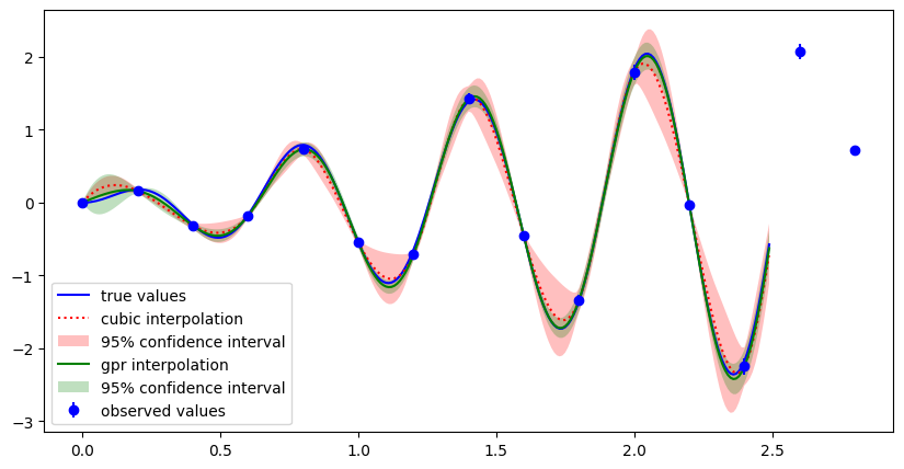
Example of 1d interpolation comparing cubic and GPR interpolation methods, as well as their uncertainties.

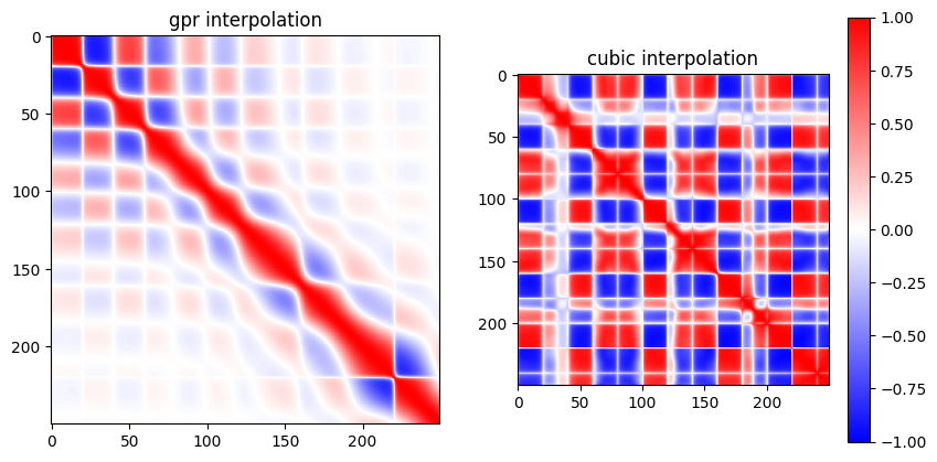
Example of error correlation matrices for cubic and GPR interpolation methods for the example in the figure above.

1D interpolation following a high-resolution example

For this use case, we have developed a method so that an interpolation can be done between a set of low resolution data points, which follows the shape of another set of high-resolution data points (or a high resolution model). This is particularly useful if the low-resolution data points have small uncertainties (and thus a good absolute calibration), while the shape of the function between the data points is known from another set of data points or model which have larger uncertainties (e.g. if we have a set of measurements with poor absolute calibration but good relative calibration). By combining these measurements, the high-resolution model can be confidently anchored to the low-resolution datapoints, thereby significantly reducing its uncertainties (especially any error-contributions that are systematic). In short, this method works by first calculating a set of residuals between the low-resolution data and high-resolution data, then interpolating these residuals to all requested wavelengths, and then combining them again with the high resolution datapoints in order to get the final interpolated datapoints. The residuals can be calculated in a relative or absolute way (depending on which is most appropriate for a given use case). The interpolation steps throughout this method use the same interpolation methods and uncertainty propagation as the normal 1D interpolation.

Below, the same example is shown where the true values lie on y=x*sin(10x), but now additionally there is some high resolution data available which has poor absolute calibration (i.e. it can be offset) but small relative uncertainties (i.e. the shape is reliable). The interpolated values and their uncertainties are shown for the cubic and gpr interpolation method. For more details we refer to this jupyter notebook.

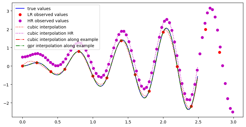
Example of 1d interpolation along an example. The high resolution data is scaled to go through the low resolution data. Uncertainties are small and the GPR and cubic methods agree well.

Extrapolation

Extrapolation is also possible using the comet_maths interpolation module. There are three options for extrapolation: “nearest”, “linear” and “extrapolate”. For “nearest”, the extrapolated values are just the nearest bounds of the provided values (i.e. constant value). For “linear”, linear extrapolation is used using the first and last two values. For “extrapolate”, the extrapolation is done using the same method as chosen for the interpolation. In this case, the extrapolation is done using built-in scipy (or sklearn for gpr) functionality. To determine the model uncertainties for extrapolation, we again have different approaches for analytical and statistical (gpr) methods, similar to the approach for the interpolation model uncertainties. For gpr, the extrapolation model uncertainty is again returned as one of the outputs of the algorithm. For the analytical methods, we again calculate the std between various cases, where now we vary between “nearest” and “extrapolate” as the extrapolation methods, while still also varying the interpolation methods. The latter also affects the extrapolated values.

When doing an interpolation along a high-resolution example, we recommend to use the “nearest” option for extrapolation. By default, the “extrapolate” option will be used when doing normal 1d interpolation, yet internally the “nearest” extrapolate option will be used by default to interpolate the residuals when interpolating along a high-resolution example. This way the high resolution data is followed as closely as possible in the regions where no low resolution data is available to constrain it.

We again show the same example where the true values lie on y=x*sin(10x), but now we are also extrapolating beyond the region for which low resolution data are available, The interpolated values and their uncertainties are shown for the cubic and gpr interpolation method. For more details we refer to this jupyter notebook.

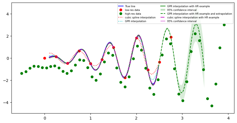
Example of 1d interpolation along an example with extrapolation. The high resolution data is scaled to go through the low resolution data. Uncertainties in the extrapolation area get progressively larger.

Usage

We here give some basic examples of usages, for further examples, we refer to this jupyter notebook.

First we give an example for normal 1D interpolation with uncertainties. The data needs to be passed as numpy arrays:

import comet_maths as cm
import numpy as np

x_measured=np.array([330.,350.,370.,390.,410.])
y_measured=np.array([10.1,12.3,14.7,16.2,18.4])
u_y_measured=np.array([0.23,0.24,0.20,0.25,0.19])

x_target=np.arange(330,400,1)

y_interpolated, u_y_interpolated, corr_y_interpolated=cm.interpolate_1d(x_measured,y_measured,x_target,u_y_i=u_y_measured,method="gpr",return_uncertainties=True,return_corr=True)

Next, we provide an example for the case where we are interpolating between low resolution data points (x_LR,y_LR) with good absolute calibration (low u_y_LR) using a high resolution example (x_HR,y_HR) with poor absolute calibration (large systematic component):

import comet_maths as cm
import numpy as np

if __name__ == '__main__':
    x_LR=np.array([330.,350.,370.,390.,410.])
    y_LR=np.array([10.1,12.3,14.7,16.2,18.4])
    u_y_LR=np.array([0.03,0.04,0.02,0.05,0.03])

    x_HR=np.arange(330,410,5)
    y_HR=np.sin(x_HR)
    u_y_HR=np.abs(y_HR*0.1) # 10% relative systematic uncertainty
    corr_y_HR=np.ones((len(y_HR),len(y_HR))) # fully systematic error-correlation matrix

    x_target=np.arange(330,400,1)

    y_interpolated, u_y_interpolated, corr_y_interpolated=cm.interpolate_1d_along_example(
        x_LR,
        y_LR,
        x_HR,
        y_HR,
        x_target,
        relative=False,
        method="cubic",
        method_hr="cubic",
        u_y_i=u_y_LR,
        corr_y_i="rand",
        u_y_hr=u_y_HR,
        corr_y_hr=corr_y_HR,
        return_uncertainties=True,
        plot_residuals=False,
        return_corr=True)

Here the “if __name__ == ‘__main__’:” is necessary (mostly on a windows machine) because the MC uncertainty propagation uses multiprocessing.